Introduction to Pandas and alternatives

Webography

Pandas tutorial
Online Doc: https://pandas.pydata.org/
CheatSheet : https://pandas.pydata.org/Pandas_Cheat_Sheet.pdf
GeoPandas : http://geopandas.org/
Pandas for SQL Users
Xarray

Import statements

Code using pandas usually starts with the import statement

import numpy as np
import pandas as pd

Pandas

2 data structures (Series, DataFrame) for data analysis
multiple methods for convenient data filtering.
toolkit utilities to perform input/output operations. It can read data from a variety of formats such as CSV, TSV, MS Excel, etc.

Pandas has two main data structures for data storage

Series
DataFrame

## Series structure
series1 = pd.Series([1, 2, 3, 4])
series1

0    1
1    2
2    3
3    4
dtype: int64

print(series1.sum())
print(series1.mean())

10
2.5

print(series1.to_csv())

,0
0,1
1,2
2,3
3,4

fruits = np.array(["kiwi", "orange", "mango", "apple"])
series2 = pd.Series(fruits)
series2

0      kiwi
1    orange
2     mango
3     apple
dtype: object

Dataframe¶

A dictionary of series where keys are column name

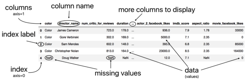
How to create a data frame ?¶

From scratch¶

# Intialise data: dictionary of lists.
data = {
    "Name": ["John", "Paul", "Debby", "Laura"],
    "Sex": ["Male", "Male", "Female", "Female"],
    "Age": [20, 40, 19, 30],
}

# Create DataFrame
df = pd.DataFrame(data)
df

type(df.Age)

pandas.core.series.Series

df.to_csv("/tmp/person.txt")

From a file¶

df_person = pd.read_csv("/tmp/person.txt", sep=",", encoding="utf-8", header=0)
df_person

By default, a new index is created

If you want use a field-based index, you have to specify it in the read_csv function:

df_person = pd.read_csv(
    "/tmp/person.txt", sep=",", index_col=0, encoding="utf-8", header=0
)
df_person

Basic commands¶

# display simple statistics
df_person.describe()

# display the 5 first rows
df_person.head()

# display the 5 last rows
df_person.tail()

# display the dataframe columns
df_person.columns

Index(['Name', 'Sex', 'Age'], dtype='object')

# query one column
df_person["Age"]

0    20
1    40
2    19
3    30
Name: Age, dtype: int64

# another method to query one column
df_person.Age

0    20
1    40
2    19
3    30
Name: Age, dtype: int64

# query multiple columns
df_person[["Name", "Age"]]

# display unique value of a column
df_person.Sex.unique()

array(['Male', 'Female'], dtype=object)

# display 2 first rows
df_person[:2]

iloc: Purely integer-location based indexing for selection by position.¶

df_person.head()

df_person.iloc[2]

Name     Debby
Sex     Female
Age         19
Name: 2, dtype: object

df_person.iloc[2, 2]

np.int64(19)

`loc`: access a group of rows and columns by label(s) or a boolean array.¶

df_person.head()

# one line
df_person.loc[2]

Name     Debby
Sex     Female
Age         19
Name: 2, dtype: object

# one value
df_person.loc[2, "Name"]

'Debby'

Basic operations on columns¶

df_person.Age = df_person.Age + 2
df_person.Age

0    22
1    42
2    21
3    32
Name: Age, dtype: int64

Get or set a single value (fast)¶

df_person.at: by labels
df_person.iat: “integer-location based indexing”

df_person.head()

df_person.at[2, "Name"]

'Debby'

df_person.iat[2, 0]

'Debby'

Add a row¶

new_row = {"Name": "Glenn", "Sex": "Male", "Age": 10}
df_person = pd.concat([df_person, pd.DataFrame([new_row])], ignore_index=True)
df_person

Add some rows¶

data = {
    "Name": ["Marguerite", "Annie", "Stephen", "Ava"],
    "Sex": ["Female", "Female", "Male", "Female"],
    "Age": [34, 23, 49, 22],
}
df_person = pd.concat([df_person, pd.DataFrame(data)], ignore_index=True)
df_person

Add a column¶

df_person["Nationality"] = "USA"
df_person

Basic statistics¶

type(df_person.Age)

pandas.core.series.Series

print(df_person.Age.mean())
print(df_person.Age.min())
print(df_person.Age.max())
print(df_person.Age.count())

28.333333333333332
10
49
9

How to sort data ?¶

df_person_sorted = df_person.sort_values(["Age"], ascending=True)
df_person_sorted

Selection¶

# selection with one criterion
df_person[df_person["Sex"] == "Female"]

df_person[df_person["Age"] < 20]

# selection with 2 criteria
df_person[(df_person["Sex"] == "Male") & (df_person["Age"] > 30)]

Update data¶

# change one value by index
df_person.loc[7, "Name"] = "Stephane"
df_person

# change one value after a selection
df_person.loc[df_person["Name"] == "Stephane", "Name"] = "Eric"
df_person

## Add a column
df_person["City"] = "City"
df_person

## Delete a column
df_person = df_person.drop("City", axis=1)
df_person

Concatenate¶

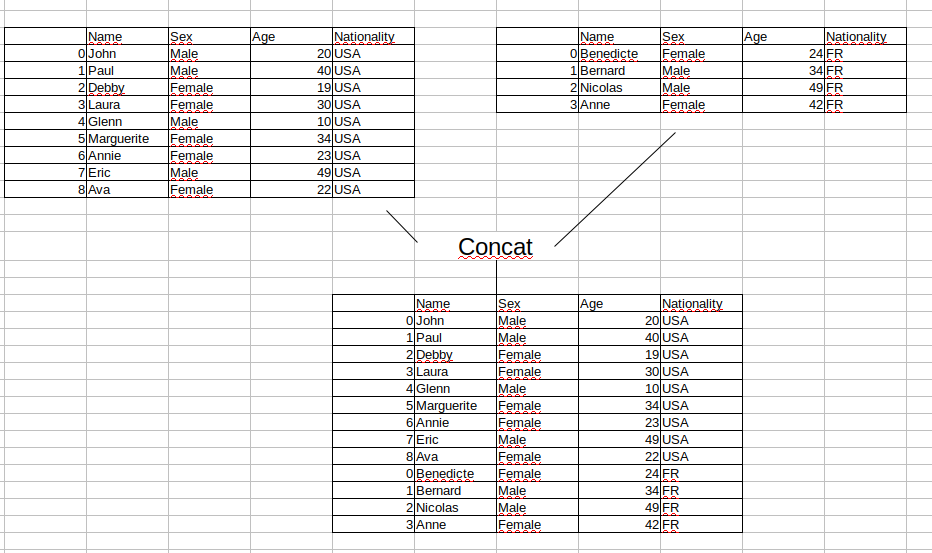
data = {
    "Name": ["Benedicte", "Bernard", "Nicolas", "Anne"],
    "Sex": ["Female", "Male", "Male", "Female"],
    "Age": [24, 34, 49, 42],
    "Nationality": ["FR", "FR", "FR", "FR"],
}
df_person_fr = pd.DataFrame(data)
list_person = [df_person, df_person_fr]
result = pd.concat(list_person)
result

Join¶

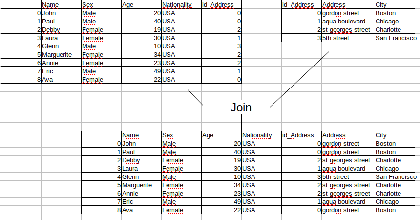
import random

data = {
    "id_Address": [0, 1, 2, 3],
    "Address": ["gordon street", "aqua boulevard", "st georges street", "5th street"],
    "City": ["Boston", "Chicago", "Charlotte", "San Francisco"],
}

# Create DataFrame
df_address = pd.DataFrame(data)
df_address

df_person["id_Address"] = ""
nb_elements = df_person.Name.count()

cpt = 0
while cpt < nb_elements:
    df_person.loc[cpt, "id_Address"] = random.randint(0, 3)
    cpt = cpt + 1
df_person

result = pd.merge(df_person, df_address, how="left", on="id_Address")
result

Group By¶

Splitting the data into groups based on some criteria.
Applying a function to each group independently.
Combining the results into a data structure.

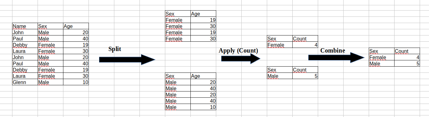
df_person.groupby("Sex")["Sex"].count()

Sex
Female    5
Male      4
Name: Sex, dtype: int64

df_person.groupby("Sex")["Age"].mean()

Sex
Female    26.40
Male      30.75
Name: Age, dtype: float64

Export data¶

export_csv = df_person.to_csv(r"/tmp/export_person.csv", index=None, header=True)

Plot data¶

%matplotlib inline

df_person.groupby("Sex")["Sex"].count().plot.bar();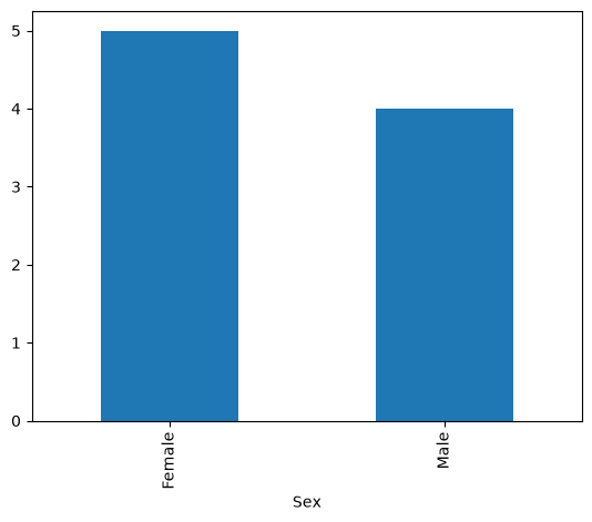

Alternatives to Pandas¶

Polar, in particular https://docs.pola.rs/user-guide/getting-started/

Dataframe¶

How to create a data frame ?¶

From scratch¶

From a file¶

Basic commands¶

iloc: Purely integer-location based indexing for selection by position.¶

loc: access a group of rows and columns by label(s) or a boolean array.¶

Basic operations on columns¶

Get or set a single value (fast)¶

Add a row¶

Add some rows¶

Add a column¶

Basic statistics¶

How to sort data ?¶

Selection¶

Update data¶

Concatenate¶

Join¶

Group By¶

Export data¶

Plot data¶

Alternatives to Pandas¶

`loc`: access a group of rows and columns by label(s) or a boolean array.¶