Practice: weather data
This section will compute statistics and observe trends in monthly weather data in the
period 1951-2023. We use real measurements from Météo-France that are available for any
region in France ( https://chamonix_weather_data_1951-2023.csv that contains data from one
of Chamonix observatories. You can use the code written previously in the previous
section where you build a weather station.
The following exercises can be either solved using only native python tools, or using specialized libraries to handle csv data. The former is better to learn python, but the latter is a lot more efficient.
Load the data
The main difference with the previous exercises is that the files are getting bigger and
treating them by hand is not a good way to proceed anymore. Still, since we are dealing
with a text file, it is a good idea to open the file and check the content. The first
line gives the name of each column, where NOM_USUEL is the location name (only Chamonix
in our case), AAAAMM is the date, RR is the rain (more precisely: cumul mensuel des
hauteurs de précipitation (en mm et 1/10)), TM the average temperature.
Solution to Exercise 1
We present two solutions, first one with dictionaries
def load_data(path, separator=";", nb_fields=4):
    """Loading the data from a file in a single dictionary"""

    station = {
        "location": [],
        "rain": [],
        "temperatures": [],
        "dates": [],
    }
    with open(path) as f:
        f.readline()
        for line in f:
            # strip the end of line
            line = line.strip("\n")
            ch = line.split(separator)

            place = ch[0]
            date = ch[1]

            station["location"].append(place)
            station["dates"].append(date)

            try:  # in case of missing data (or corrupt), discard the full line
                rain = float(ch[2])
                temperature = float(ch[3])
            except ValueError:
                # save data
                station["rain"].append(np.nan)
                station["temperatures"].append(np.nan)

            # save data
            station["rain"].append(rain)
            station["temperatures"].append(temperature)

    return station


path = f"../common/data_read_files/chamonix_weather_data_1951-2023.csv"
station = load_data(path)
and a second with classes
import numpy as np
import pandas as pd
from pathlib import Path


class WeatherStation:
    """A weather station that holds weather data, namely

    - dates
    - location
    - rain
    - temperatures
    """

    def __init__(self, name: str, dates, location, rain, temperatures):
        """initialize the weather station."""
        self.name = name
        self.dates = dates
        self.location = location
        self.rain = rain
        self.temperatures = temperatures

    @classmethod
    def from_csv(cls, filename: str, name: str, sep=";") -> Self:
        """
        loads a csv filename using the fields
            NOM_USUEL       : nom usuel du poste
            AAAAMM          : mois
            RR              : cumul mensuel des hauteurs de précipitation (en mm et 1/10)
            TM              : moyenne mensuelle des (TN+TX)/2 quotidiennes (en °C et 1/10)
        raise RuntimeError if import fails
        :filename: str|Path
        :returns: None
        """
        df = pd.read_csv(filename, sep=sep)

        # change date to a more convenient format
        df["dates"] = pd.to_datetime(df.AAAAMM, format="%Y%m")

        location = df["NOM_USUEL"]
        rain = df["RR"]
        temperatures = df["TM"]

        return WeatherStation(name, df["dates"], location, rain, temperatures)


path = "../common/data_read_files/chamonix_weather_data_1951-2023.csv"
chamonix = WeatherStation.from_csv(path, "Chamonix")
Compute statistics
Solution to Exercise 2
# convert numerical data to numpy arrays
for key in ["rain", "temperatures"]:
    station["rain"] = np.array(station["rain"])
    station["temperatures"] = np.array(station["temperatures"])

# Check that there is no nans values
nans_mask = np.isnan(station["temperatures"])
print("invalid values:", np.sum(nans_mask))

# compute average on all values
avg_temp = np.mean(station["temperatures"])
sigma_temp = np.std(station["temperatures"])
print(f"Average temperature (1951-2023): {avg_temp:.2f} +/- {sigma_temp:.2f} °C")

# slicing does not work (i.e. station['rain'][5::12]) if there are missing elements!
# Instead, one should look for dates that finish with 6
june_rain = station["rain"][5::12]  # take every 12 elements, starting in june
print(f"Average rain in june (1951-2023): {np.mean(june_rain):.2f} mm")

# find indices when rain is superior to 100mm
heavy_rain_months = station["rain"] > 100
temp_when_raining = np.mean(station["temperatures"][heavy_rain_months])
print(f"Average temp in rainy months (1951-2023): {temp_when_raining:.2f} °C")
invalid values: 0
Average temperature (1951-2023): 7.12 +/- 6.91 °C
Average rain in june (1951-2023): 122.78 mm
Average temp in rainy months (1951-2023): 8.04 °C
With the oriented object and pandas
# compute average on all values but nans
avg_temp = chamonix.temperatures.mean()
sigma_temp = chamonix.temperatures.std()
print(f"Average temperature (1951-2023): {avg_temp:.2f} +/- {sigma_temp:.2f} °C")

# use pandas datetime to get something clearer than Numpy
june_rain = chamonix.rain[chamonix.dates.dt.month == 6]
print(f"Average rain in june (1951-2023): {np.mean(june_rain):.2f} mm")

# find indices when rain is superior to 100mm
heavy_rain_months = chamonix.rain > 100
temp_when_raining = chamonix.temperatures[heavy_rain_months].mean()
print(f"Average temp in rainy months (1951-2023): {temp_when_raining:.2f} °C")
Average temperature (1951-2023): 7.12 +/- 6.91 °C
Average rain in june (1951-2023): 122.78 mm
Average temp in rainy months (1951-2023): 8.04 °C
Climate evolution
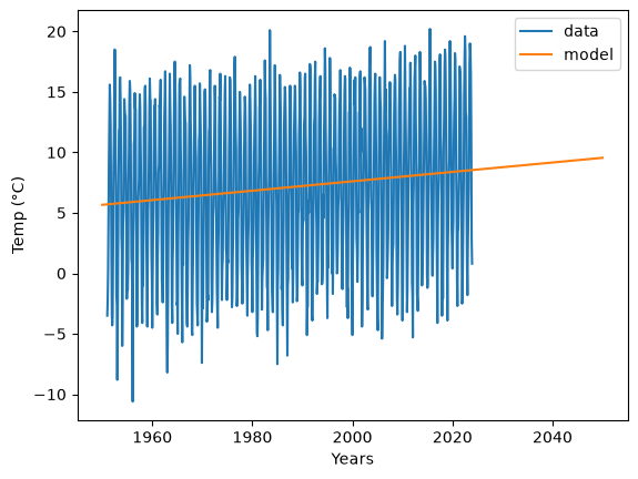
We now turn to the more interesting part, we compute how temperatures increased in Chamonix. Then we model the temperatures to make a prediction for 2050.
Solution to Exercise 3
For both approaches, we need to convert the dates to numerical values
# convert dates to numerical values
years = [int(d[:4]) for d in station["dates"]]  # years correspond to 4 first characters
months = [
    int(d[4:]) for d in station["dates"]
]  # months correspond to 2 last characters
station["numerical_dates"] = np.array(years) + (np.array(months) - 1) / 12
And for pandas
# convert dates to numerical values
numerical_dates = chamonix.dates.dt.year + (chamonix.dates.dt.month - 1) / 12
temperatures = chamonix.temperatures
The rest of the exercise can be done in the same way
import matplotlib.pyplot as plt

fig, ax = plt.subplots()

ax.set_xlabel("Years")
ax.set_ylabel("Temp (°C)")
ax.plot(numerical_dates, temperatures);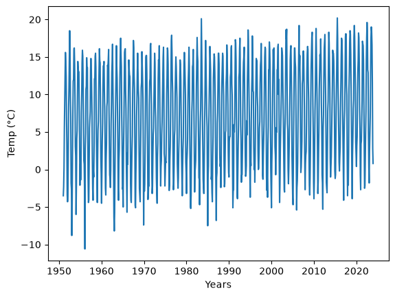
from scipy.optimize import curve_fit


def linear(dates, slope, intercept):
    return slope * dates + intercept


# we fit the model
opt_params, pcov = curve_fit(
    linear,
    numerical_dates,
    temperatures,
)
slope, intercept = opt_params

# important, test if the model fit the data
# since this is a line, we only need two points

fig, ax = plt.subplots()


ax.plot(numerical_dates, temperatures, label="data")  # plot the data for reference
times = [1950, 2050]
temps_model = [slope * time + intercept for time in times]
ax.set_xlabel("Years")
ax.set_ylabel("Temp (°C)")
ax.plot(times, temps_model, label="model")
plt.legend()

print(f"temperature change {slope * 100:.2f} °C / 100 year")
print(f"Average temperature in 2050 {temps_model[1]:.2f} °C")
temperature change 3.89 °C / 100 year
Average temperature in 2050 9.55 °C
Final comment: The exercises could be solved with either pandas or numpy. However the two librairies have different scopes. To read CSV files, compute means, or handle dates pandas offer a simpler interface. However to perform more complex mathematical operations such as linear algebra operations, numpy is a better choice. Furthermore, numpy arrays are handled by a variety of other librairies (e.g. scipy). In practice, you can of course use both librairies, depending on the task. If you want to redo the exercise with other stations, which will likely have missing data, the simplest way is to use pandas.